Dimensionality Reduction

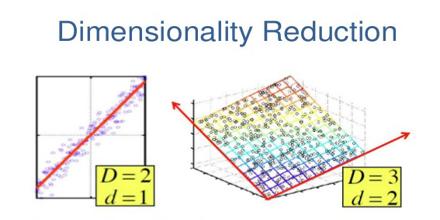
We can not visualize our data which has more than three dimension. For the data with only one dimension, we can make a line plot. For two dimensional data, we can plot a two dimensional graph, For three dimensional data, we add a more axis Z with other two, X-Y axis to visualize how the data is distributed. Visualization is the key technique in this field. So for higher than three dimensional data, we can not make any plot. It is  very challenging to us to visualize such higher dimensional data. Again, Machine Learning models also have a tendency of lowering accuracy  with increase in dimension i.e. no. of independent variables. It means when we have higher dimensional data then we have to somehow reduce the no. of dimension. This process by which we can reduce higher dimensional data to lower dimension  is called Dimension reduction.

In the above picture, right side image with higher(3) dimension is transformed into lower(2) dimension.

What is 'Dimension Reduction'?

Dimensionality reduction, also known as Dimension Reduction, is a transformation technique so that higher dimension space can be represented by low dimension space with very minimal loss of information, ideally 0. There are many techniques by which we can reduce higher dimensional data to lower dimensional data. 

Techniques for 'Dimension reduction'

There are many ways to reduce higher dimensional data. such as-

• Neglecting the variables which has some linear dependency [ By checking the correlation factor ] 

Corr(X,Y) = R = Coefficient of Correlation

• Though in some cases correlation factor is 0, but there can present some complex relationship between them. Then also we can neglect one of them. let's have a look the picture.

Some relationship is there but R value is 0

• Using strong domain knowledge, we can also reduce dimension. But it takes a lot of effort.
• We need some general method to reduce the dimension of the data. That is why we use PCA( Principal Component Analysis ). This algorithm is based on Eigen Value and associated Eigen Vector.

PCA

It is a process by which we can get the Principal Component(s)(PCs) present in the higher dimensional data. The maximum number of Principal component present is equal to the total no. of  independent variables present.

•  First we calculate the Eigen value for each  independent variable. 
• we sort  those Eigen Values over magnitude in decreasing order. 
• The direction of the PC( Principal Component ), calculated using Eigen Vector, is given by the associated Eigen Vector.
• Then we decide the number of components present by Scree Plot, based on variance ratio of the points
• Then the points are projected on those PCs.
• The projected value now used for further analysis.

Python code

• First import the required library

• Then creating a data-frame

• Then setting no. of components = total no of independent variables i.e. 4 and plotting the scree plot to see which component(s) is/are dominant.

• We can clearly see that the first principal components is the dominant component and explains information of the original data about the >90%.

Now we can do further analysis with the first principal component and the 'species' column of the main data-frame.

Conclusion

In this post we have shown about the Dimensionality Reduction and also some techniques to deal in such scenario. At last we have shown PC analysis in python and about the scree plot which gives us the measure of variation of data from the original data.